2022-07-20 mysql-hashJoin说明

hash join describe

Hash Join

The hash join algorithm is a very recent addition to MySQL and is supported in MySQL

8.0.18 and later. It marks a significant break with the tradition of nested loop joins

including the block nested loop variant. It is particularly useful for large joins without

indexes but can in some cases even outperform an index join.

MySQL implements a hybrid between a classic in-memory hash join and the on-disk

GRACE hash join algorithm. 2 If it is possible to store all the hashes in memory, then the

pure in-memory implementation is used. The join buffer is used for the in-memory part,

so the amount of memory that can be used for the hashes is limited by join_buffer_

size . When the join does not fit in memory, the join spills over to disk, but the actual

join operations are still performed in memory.

The in-memory hash join algorithm consists of two steps:

1. One of the tables in the join is chosen as the build table . The hash

is calculated for the columns required for the join and loaded into

memory. This is known as the build phase .

2. The other table in the join is the probe input . For this table, rows

are read one at a time, and the hash is calculated. Then a hash

key lookup is performed on the hashes calculated from the build

table, and the result of the join is generated from the matching

rows. This is known as the probe phase .

When the hashes of the build table do not fit into memory, MySQL automatically

switches to use the on-disk implementation (based on the GRACE hash join algorithm).

The switch from the in-memory to the on-disk algorithm happens if the join buffer

becomes full during the build phase. The on-disk algorithm consists of three steps:

1. Calculate the hashes of all rows in both the build and probe tables

and store them on disk in several small files partitioned by the

hash. The number of partitions is chosen to make each partition

of the probe table fit into the join buffer but with a limit of at most

128 partitions.

2. Load the first partition of the build table into memory and iterate

over the hashes from the probe table in the same way as for the

probe phase for the in-memory algorithm. Since the partitioning

in step 1 uses the same hash function for both the build and probe

tables, it is only necessary to iterate over the first partition of the

probe table.

3. Clear the in-memory buffer and continue with the rest of the

partitions one by one.

Both the in-memory and on-disk algorithms use the xxHash64 hash function which

is known as being fast while still providing hashes of good quality (reducing the number

of hash collisions). For the optimal performance, the join buffer needs to be large

enough to fit all the hashes from the build table. That said, the same considerations for

join_buffer_size exist for hash joins as for block nested loop joins.

MySQL will use the hash join whenever the block nested loop would otherwise be

chosen, and the hash join algorithm is supported for the query. At the time of writing,

the following requirements exist for the hash join algorithm to be used:

• The join must be an inner join.

• The join cannot be performed using an index, either because there is

no available index or because the indexes have been disabled for the

query.

• All joins in the query must have at least one equi-join condition

between the two tables in the join, and only columns from the two

tables as well as constants are referenced in the condition.

• As of 8.0.20, anti, semi, and outer joins are also supported. 3 If you join

the two tables t1 and t2 , then examples of join conditions that are

supported for hash join include

• t1.t1_val = t2.t2_val

• t1.t1_val = t2.t2_val + 2

• t1.t1_val1 = t2.t2_val AND t1.t1_val2 > 100

• MONTH(t1.t1_val) = MONTH(t2.t2_val)

If you consider the recurring example query for this section, you can execute it using

a hash join by ignoring the indexes on the tables that can be used for the join:

SELECT CountryCode, country.Name AS Country,

city.Name AS City, city.District

FROM world.country IGNORE INDEX (Primary)

INNER JOIN world.city IGNORE INDEX (CountryCode)

ON city.CountryCode = country.Code

WHERE Continent = 'Asia';

The pseudo code for performing this join is similar to that of a block nested loop

except that the columns needed for the join are hashed and that there is support for

overflowing to disk.

result = []
join_buffer = []
partitions = 0
on_disk = False
for country_row in country:
 if country_row.Continent == 'Asia':
 hash = xxHash64(country_row.Code)
 if not on_disk:
 join_buffer.append(hash)
 if is_full(join_buffer):
 # Create partitions on disk
 on_disk = True
 partitions = write_buffer_to_disk(join_buffer)
 join_buffer = []
 else
 write_hash_to_disk(hash)
if not on_disk:
 for city_row in city:
 hash = xxHash64(city_row.CountryCode)
 if hash in join_buffer:
 country_row = get_row(hash)
 city_row = get_row(hash)
 result.append(join_rows(country_row, city_row))
else:
 for city_row in city:
 hash = xxHash64(city_row.CountryCode)
 write_hash_to_disk(hash)
 for partition in range(partitions):
 join_buffer = load_build_from_disk(partition)
 for hash in load_hash_from_disk(partition):
if hash in join_buffer:
 country_row = get_row(hash)
 city_row = get_row(hash)
 result.append(join_rows(country_row, city_row))
 join_buffer = []

The pseudo code starts out reading the rows from the country table and calculates

the hash for the Code column and stores it in the join buffer. If the buffer becomes full,

then the code switches to the on-disk algorithm and writes out the hashes from the

buffer. This is also where the number of partitions is determined. After this the rest of the

country table is hashed.

In the next part, for the in-memory algorithm, there is a simple loop over the rows in

the city table comparing the hashes to those in the buffer. For the on-disk algorithm, the

hashes of the city table are first calculated and stored on disk; then the partitions are

handled one by one.

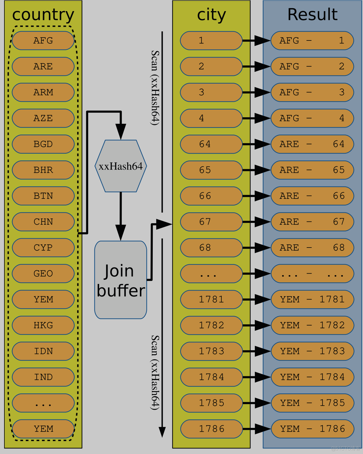
The values of the Code column for the matching rows from the country table are

hashed and stored in the join buffer. Then a table scan is executed for the city table with

the hash calculated of CountryCode for each row, and the result is constructed from the

matching rows.

You can see the query performs very well with the hash join examining the same

number of rows as the block nested loop, but it is faster than an index join. This is not a

mistake: in some cases, a hash join can outperform even an index join. You can use the

following rules to estimate how the hash join algorithm will perform compared to index

and block nested loop joins:

• For a join without using an index, the hash join will usually be much

faster than a block nested join unless a LIMIT clause has been added.

Improvements of more than a factor of 1000 have been observed. 4

• For a join without an index where there is a LIMIT clause, a block

nested loop can exit when enough rows have been found, whereas

a hash join will complete the entire join (but can skip fetching the

rows). If the number of rows included due to the LIMIT clause is small

compared to the total number of rows found by the join, a block

nested loop may be faster.

• For joins supporting an index, the hash join algorithm can be faster if

the index has a low selectivity.

The biggest benefit using the hash joins is by far for joins without an index and

without a LIMIT clause. In the end, only testing can prove which join strategy is the

optimal for your queries.

You can enable and disable support for hash joins using the hash_join optimizer

switch. Additionally, the block_nested_loop optimizer switch must be enabled. Both are

enabled by default. If you want to configure the use of hash joins for specific joins, you

can use the HASH_JOIN() and NO_HASH_JOIN() optimizer hints.

That concludes the discussion about the three high-level join strategies supported in

MySQL.There are some lower-level optimizations as well that are worth considering.