 云计算服务
云计算服务
 服务器租用
服务器租用
 DDOS 防护
 虚拟主机
虚拟主机
 域名服务
域名服务
 基础设施
基础设施
 关于我们
关于我们
Consider the task of driving an underpowered car up a steep mountain road. The diculty is that gravity is stronger than the car’s engine, and even at full throttle the car cannot accelerate up the steep slope. The only solution is to first move away from the goal and up the opposite slope on the left. Then, by applying full throttle the car can build up enough inertia to carry it up the steep slope even though it is slowing down the whole way. This is a simple example of a continuous control task where things have to get worse in a sense (farther from the goal) before they can get better. Many control methodologies have great diculties with tasks of this kind unless explicitly aided by a human designer. Consider the task of driving an underpowered car up a steep mountain road. The diculty is that gravity is stronger than the car’s engine, and even at full throttle the car cannot accelerate up the steep slope. The only solution is to first move away from the goal and up the opposite slope on the left. Then, by applying full throttle the car can build up enough inertia to carry it up the steep slope even though it is slowing down the whole way. This is a simple example of a continuous control task where things have to get worse in a sense (farther from the goal) before they can get better. Many control methodologies have great diculties with tasks of this kind unless explicitly aided by a human designer.
2 部分代码% This is the main file for the simulation.
clear

close all
clc
%% Set simulation parameters.
% There is a minimum grid size here. Otherwise, traceBack function will
% fail. Since the dynamic equation of the car is:
% vNext = v + 0.001 * u - 0.0025 * cos(3 * p);
% When v(0) = 0, and cos(3p) = 0, u = 1, will result in vNext = 0.001. For
% this reason, velocity grid should be finer that 0.001.
% Bigger number means finer grids
% We will create a grid/matrix, the row is for the discretized position and
% the column is for the discretized velocity.
gridSizePos = 400;
gridSizeVel = 400;
% x0 holds the initial position and velocity;
% Select -0.6 to -0.4 for position.
% Initial velocity shold be zero as described in the original problem.
x0 = [-0.52 0];
%x0 = [0.4 0];
%% Find optimal policy.
tic
[error, predecessorP, predecessorV, policy] = ...
mountainCarValIter(gridSizePos, gridSizeVel, 1000);
toc
%% Trace back the optimal policy, for given a certain initial condition
[XStar, UStar, TStar] = ...
traceBack(predecessorP, predecessorV, policy, x0, gridSizePos, gridSizeVel);
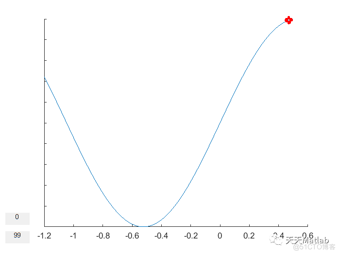
%% Animation
visualizeMountainCar(gridSizePos, XStar, UStar)
%% Plot errors over iterations.
figure
plot(error);
title('Convergence errors over iterations');
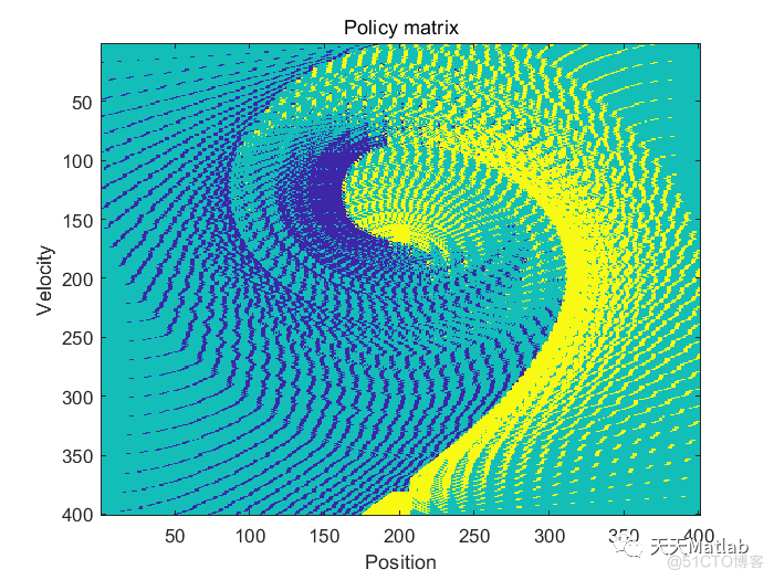
%% Plot the policy matrix.
figure
imagesc(policy)
title('Policy matrix')
xlabel('Position');
ylabel('Velocity');
3 运行结果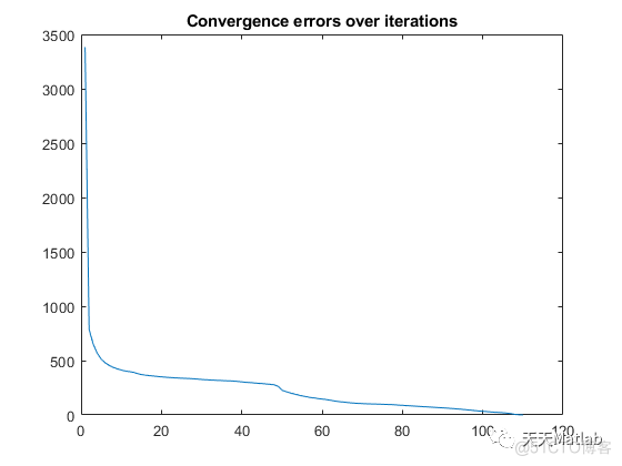


.png)

.png)

