 云计算服务
云计算服务
 服务器租用
服务器租用
 DDOS 防护
 虚拟主机
虚拟主机
 域名服务
域名服务
 基础设施
基础设施
 关于我们
关于我们
我们基于以下三条数据预测了加州大学洛杉矶分校 (UCLA) 的研究生录取情况:
GRE 分数(测试)即 GRE Scores (Test)GPA 分数(成绩)即 GPA Scores (Grades)评级(1-4)即 Class rank (1-4)数据集来源: http://www.ats.ucla.edu/

为了加载数据并很好地进行格式化,我们将使用两个非常有用的包,即 Pandas 和 Numpy。 你可以在这里阅读文档:
https://pandas.pydata.org/pandas-docs/stable/https://docs.scipy.org/# Importing pandas and numpy
import pandas as pd
import numpy as np
# Reading the csv file into a pandas DataFrame
data = pd.read_csv('student_data.csv')
# Printing out the first 10 rows of our data
data[:10]
admit
gre
gpa
rank
0
0
380
3.61
3
1
1
660
3.67
3
2
1
800
4.00
1
3
1
640
3.19
4
4
0
520
2.93
4
5
1
760
3.00
2
6
1
560
2.98
1
7
0
400
3.08
2
8
1
540
3.39
3
9
0
700
3.92
2
首先让我们对数据进行绘图,看看它是什么样的。为了绘制二维图,让我们先忽略评级 (rank)。
# Importing matplotlib
import matplotlib.pyplot as plt
%matplotlib inline
# Function to help us plot
def plot_points(data):
    X = np.array(data[["gre","gpa"]])
    y = np.array(data["admit"])
    admitted = X[np.argwhere(y==1)]
    rejected = X[np.argwhere(y==0)]
    plt.scatter([s[0][0] for s in rejected], [s[0][1] for s in rejected], s = 25, color = 'red', edgecolor = 'k')
    plt.scatter([s[0][0] for s in admitted], [s[0][1] for s in admitted], s = 25, color = 'cyan', edgecolor = 'k')
    plt.xlabel('Test (GRE)')
    plt.ylabel('Grades (GPA)')

# Plotting the points
plot_points(data)
plt.show()
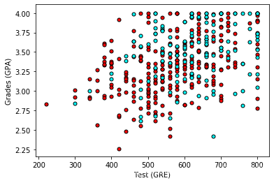
粗略来说,它看起来像是,成绩 (grades) 和测试 (test) 分数高的学生通过了,而得分低的学生却没有,但数据并没有如我们所希望的那样,很好地分离。 也许将评级 (rank) 考虑进来会有帮助? 接下来我们将绘制 4 个图,每个图代表一个级别。
# Separating the ranks
data_rank1 = data[data["rank"]==1]
data_rank2 = data[data["rank"]==2]
data_rank3 = data[data["rank"]==3]
data_rank4 = data[data["rank"]==4]

# Plotting the graphs
plot_points(data_rank1)
plt.title("Rank 1")
plt.show()
plot_points(data_rank2)
plt.title("Rank 2")
plt.show()
plot_points(data_rank3)
plt.title("Rank 3")
plt.show()
plot_points(data_rank4)
plt.title("Rank 4")
plt.show()
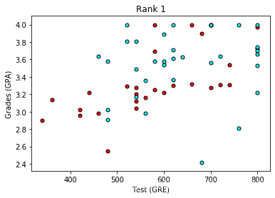
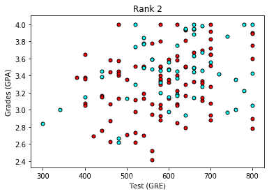
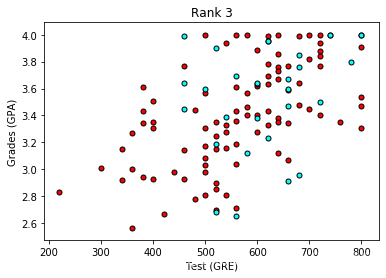
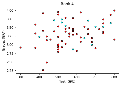
现在看起来更棒啦,看上去评级越低,录取率越高。 让我们使用评级 (rank) 作为我们的输入之一。 为了做到这一点,我们应该对它进行一次one-hot 编码。
将评级进行 One-hot 编码我们将在 Pandas 中使用 get_dummies 函数。
# Make dummy variables for rank
one_hot_data = pd.concat([data, pd.get_dummies(data['rank'], prefix='rank')], axis=1)
one_hot_data[:10]
admit
gre
gpa
rank
rank_1
rank_2
rank_3
rank_4
0
0
380
3.61
3
0
0
1
0
1
1
660
3.67
3
0
0
1
0
2
1
800
4.00
1
1
0
0
0
3
1
640
3.19
4
0
0
0
1
4
0
520
2.93
4
0
0
0
1
5
1
760
3.00
2
0
1
0
0
6
1
560
2.98
1
1
0
0
0
7
0
400
3.08
2
0
1
0
0
8
1
540
3.39
3
0
0
1
0
9
0
700
3.92
2
0
1
0
0
# Drop the previous rank column
one_hot_data = one_hot_data.drop('rank', axis=1)

# Print the first 10 rows of our data
one_hot_data[:10]
admit
gre
gpa
rank_1
rank_2
rank_3
rank_4
0
0
380
3.61
0
0
1
0
1
1
660
3.67
0
0
1
0
2
1
800
4.00
1
0
0
0
3
1
640
3.19
0
0
0
1
4
0
520
2.93
0
0
0
1
5
1
760
3.00
0
1
0
0
6
1
560
2.98
1
0
0
0
7
0
400
3.08
0
1
0
0
8
1
540
3.39
0
0
1
0
9
0
700
3.92
0
1
0
0
下一步是缩放数据。 我们注意到成绩 (grades) 的范围是 1.0-4.0,而测试分数 (test scores) 的范围大概是 200-800,这个范围要大得多。 这意味着我们的数据存在偏差,使得神经网络很难处理。 让我们将两个特征放在 0-1 的范围内,将分数除以 4.0,将测试分数除以 800。
# Making a copy of our data
processed_data = one_hot_data[:]

# TODO: Scale the columns
processed_data['gre'] = processed_data['gre']/800

processed_data['gpa'] = processed_data['gpa']/800

# Printing the first 10 rows of our procesed data
processed_data[:10]
admit
gre
gpa
rank_1
rank_2
rank_3
rank_4
0
0
0.475
0.004513
0
0
1
0
1
1
0.825
0.004587
0
0
1
0
2
1
1.000
0.005000
1
0
0
0
3
1
0.800
0.003987
0
0
0
1
4
0
0.650
0.003663
0
0
0
1
5
1
0.950
0.003750
0
1
0
0
6
1
0.700
0.003725
1
0
0
0
7
0
0.500
0.003850
0
1
0
0
8
1
0.675
0.004237
0
0
1
0
9
0
0.875
0.004900
0
1
0
0
为了测试我们的算法,我们将数据分为训练集和测试集。 测试集的大小将占总数据的 10%。
sample = np.random.choice(processed_data.index, size=int(len(processed_data)*0.9), replace=False)
train_data, test_data = processed_data.iloc[sample], processed_data.drop(sample)

print("Number of training samples is", len(train_data))
print("Number of testing samples is", len(test_data))
print(train_data[:10])
print(test_data[:10])
Number of training samples is 360将数据分成特征和目标(标签)
Number of testing samples is 40
admit gre gpa rank_1 rank_2 rank_3 rank_4
7 0 0.500 0.003850 0 1 0 0
9 0 0.875 0.004900 0 1 0 0
165 0 0.875 0.005000 1 0 0 0
158 0 0.825 0.004363 0 1 0 0
211 0 0.725 0.003775 0 1 0 0
327 1 0.700 0.004350 0 1 0 0
132 0 0.725 0.004250 0 1 0 0
151 0 0.500 0.004225 0 1 0 0
78 0 0.675 0.003900 1 0 0 0
350 1 0.975 0.005000 0 1 0 0
admit gre gpa rank_1 rank_2 rank_3 rank_4
13 0 0.875 0.003850 0 1 0 0
15 0 0.600 0.004300 0 0 1 0
18 0 1.000 0.004687 0 1 0 0
21 1 0.825 0.004537 0 1 0 0
30 0 0.675 0.004725 0 0 0 1
54 0 0.825 0.004175 0 0 1 0
55 1 0.925 0.005000 0 0 1 0
56 0 0.700 0.003987 0 0 1 0
66 0 0.925 0.004525 0 0 0 1
69 0 1.000 0.004662 1 0 0 0
现在,在培训前的最后一步,我们将把数据分为特征 (features)(X)和目标 (targets)(y)。
features = train_data.drop('admit', axis=1)
targets = train_data['admit']
features_test = test_data.drop('admit', axis=1)
targets_test = test_data['admit']

print(features[:10])
print(targets[:10])
gre gpa rank_1 rank_2 rank_3 rank_4训练二层神经网络
7 0.500 0.003850 0 1 0 0
9 0.875 0.004900 0 1 0 0
165 0.875 0.005000 1 0 0 0
158 0.825 0.004363 0 1 0 0
211 0.725 0.003775 0 1 0 0
327 0.700 0.004350 0 1 0 0
132 0.725 0.004250 0 1 0 0
151 0.500 0.004225 0 1 0 0
78 0.675 0.003900 1 0 0 0
350 0.975 0.005000 0 1 0 0
7 0
9 0
165 0
158 0
211 0
327 1
132 0
151 0
78 0
350 1
Name: admit, dtype: int64
已经准备数据,现在我们来训练一个简单的两层神经网络:
首先,我们将写一些 helper 函数。
# Activation (sigmoid) function误差反向传播
def sigmoid(x):
return 1 / (1 + np.exp(-x))
def sigmoid_prime(x):
return sigmoid(x) * (1-sigmoid(x))
def error_formula(y, output):
return - y*np.log(output) - (1 - y) * np.log(1-output)
现在轮到你来练习,编写误差项。 记住这是由方程
# TODO: Write the error term formula
def error_term_formula(y, output):
    return (y-output)
# Neural Network hyperparameters
epochs = 1000
learnrate = 0.5

# Training function
def train_nn(features, targets, epochs, learnrate):

    # Use to same seed to make debugging easier
    np.random.seed(42)

    n_records, n_features = features.shape
    last_loss = None

    # Initialize weights
    weights = np.random.normal(scale=1 / n_features**.5, size=n_features)
    print(weights.shape)


    for e in range(epochs):
        del_w = np.zeros(weights.shape)
        for x, y in zip(features.values, targets):
            # Loop through all records, x is the input, y is the target

            # Activation of the output unit
            #   Notice we multiply the inputs and the weights here
            #   rather than storing h as a separate variable
            output = sigmoid(np.dot(x, weights))

            # The error, the target minus the network output
            error = error_formula(y, output)

            # The error term
            #   Notice we calulate f'(h) here instead of defining a separate
            #   sigmoid_prime function. This just makes it faster because we
            #   can re-use the result of the sigmoid function stored in
            #   the output variable
            error_term = error_term_formula(y, output)
            #print("error_term:",error_term)

            # The gradient descent step, the error times the gradient times the inputs
            del_w += error_term * x

        # Update the weights here. The learning rate times the
        # change in weights, divided by the number of records to average
        weights += learnrate * del_w / n_records

        # Printing out the error on the training set
        if e % (epochs / 10) == 0:
            out = sigmoid(np.dot(features, weights))
            #print(out)
            loss = np.mean((out - targets) ** 2)
            print("Epoch:", e)
            if last_loss and last_loss < loss:
                print("Train loss: ", loss, "  WARNING - Loss Increasing")
            else:
                print("Train loss: ", loss)
            last_loss = loss
            print("=========")
    print("Finished training!")
    return weights

weights = train_nn(features, targets, epochs, learnrate)
(6,)计算测试 (Test) 数据的精确度
Epoch: 0
Train loss: 0.273075830588848
=========
Epoch: 100
Train loss: 0.20520354225199638
=========
Epoch: 200
Train loss: 0.20393525728827555
=========
Epoch: 300
Train loss: 0.2030136874864369
=========
Epoch: 400
Train loss: 0.2022100443775751
=========
Epoch: 500
Train loss: 0.2015047057211576
=========
Epoch: 600
Train loss: 0.20088633117322183
=========
Epoch: 700
Train loss: 0.2003443983488469
=========
Epoch: 800
Train loss: 0.1998693847500299
=========
Epoch: 900
Train loss: 0.19945286989297628
=========
Finished training!
# Calculate accuracy on test data
tes_out = sigmoid(np.dot(features_test, weights))
predictions = tes_out > 0.5
accuracy = np.mean(predictions == targets_test)
print("Prediction accuracy: {:.3f}".format(accuracy))
Prediction accuracy: 0.675
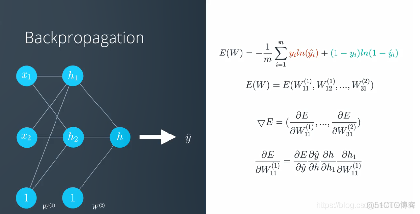
对于深度神经网络(多层神经网络),原理相同,需要通过链式法则,将错误函数反向传播到每层网络的对应节点,调整参数


.png)

.png)

