斯坦福CS231n项目实战（二）：线性支持向量机SVM

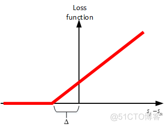
支持向量机(Support Vector Machine, SVM)的目标是希望正确类别样本的分数(WTX W T X )比错误类别的分数越大越好。两者之间的最小距离(margin)我们用Δ Δ 来表示，一般令Δ=1 Δ = 1 。

对于单个样本，SVM的Loss function可表示为：

Li=∑j≠yimax(0,sj−syi+Δ) L i = ∑ j ≠ y i m a x ( 0 , s j − s y i + Δ )

将sj=WTjxi s j = W j T x i ，syi=WTyixi s y i = W y i T x i 带入上式：

Li=∑j≠yimax(0,WTjxi−WTyixi+Δ) L i = ∑ j ≠ y i m a x ( 0 , W j T x i − W y i T x i + Δ )

其中，(xi,yi) ( x i , y i ) 表示正确类别，syi s y i 表示正确类别的分数score，sj s j 表示错误类别的分数score。从Li L i 表达式来看，sj s j 不仅要比syi s y i 小，而且距离至少是Δ Δ ，才能保证Li=0 L i = 0 。若sj>syi+Δ s j > s y i + Δ ，则Li>0 L i > 0 。也就是说SVM希望sj s j 与syi s y i 至少相差一个Δ Δ 的距离。

该Loss function我们称之为Hinge Loss:

举个简单的例子，假如一个三分类的输出分数为：[10, 20, -10]，正确的类别是第0类，则该样本的Loss function为：

Li=max(0,20−10+1)+max(0,−10−10+1)=11 L i = m a x ( 0 , 20 − 10 + 1 ) + m a x ( 0 , − 10 − 10 + 1 ) = 11

若正确的类别是第1类，则Loss function为：

Li=max(0,10−20+1)+max(0,−10−20+1)=0 L i = m a x ( 0 , 10 − 20 + 1 ) + m a x ( 0 , − 10 − 20 + 1 ) = 0

值得一提的是，还可以对hinge loss进行平方处理，也称为L2-SVM。其Loss function为：

Li=∑j≠yimax(0,WTjxi−WTyixi+Δ)2 L i = ∑ j ≠ y i m a x ( 0 , W j T x i − W y i T x i + Δ ) 2

这种平方处理的目的是增大对正类别与负类别之间距离的惩罚。

为了防止过拟合，限制权重Ｗ的大小，引入正则项：

Li=∑j≠yimax(0,WTjxi−WTyixi+Δ)+λ∑k∑lW2k,l L i = ∑ j ≠ y i m a x ( 0 , W j T x i − W y i T x i + Δ ) + λ ∑ k ∑ l W k , l 2

L2正则项作用是限制权重W过大，且使得权重W分布均匀。而L1正则项倾向于得到离散的W，各W之间差距较大。

下面是Linear SVM的实例代码，本文详细代码请见我的：

# Load the raw CIFAR-10 data.
cifar10_dir = 'CIFAR10/datasets/cifar-10-batches-py'
X_train, y_train, X_test, y_test = load_CIFAR10(cifar10_dir)

# As a sanity check, we print out the size of the training and test data.
print('Training data shape: ', X_train.shape)
print('Training labels shape: ', y_train.shape)
print('Test data shape: ', X_test.shape)
print('Test labels shape: ', y_test.shape)

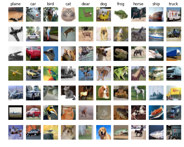
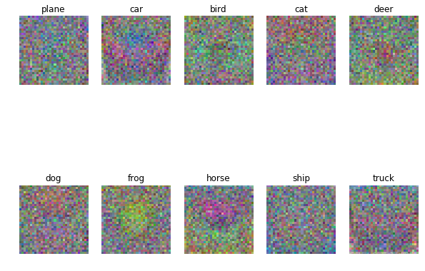
Training data shape:  (50000, 32, 32, 3)
Training labels shape:  (50000,)
Test data shape:  (10000, 32, 32, 3)
Test labels shape:  (10000,)

classes = ['plane', 'car', 'bird', 'cat', 'dear', 'dog', 'frog', 'horse', 'ship', 'truck']
num_classes = len(classes)
num_each_class = 7

for y, cls in enumerate(classes):
    idxs = np.flatnonzero(y_train == y)
    idxs = np.random.choice(idxs, num_each_class, replace=False)
    for i, idx in enumerate(idxs):
        plt_idx = i * num_classes + (y + 1)
        plt.subplot(num_each_class, num_classes, plt_idx)
        plt.imshow(X_train[idx].astype('uint8'))
        plt.axis('off')
        if i == 0:
            plt.title(cls)
plt.show()

# Split the data into train, val, and test sets
num_train = 49000
num_val = 1000
num_test = 1000

# Validation set
mask = range(num_train, num_train + num_val)
X_val = X_train[mask]
y_val = y_train[mask]

# Train set
mask = range(num_train)
X_train = X_train[mask]
y_train = y_train[mask]

# Test set
mask = range(num_test)
X_test = X_test[mask]
y_test = y_test[mask]

print('Train data shape: ', X_train.shape)
print('Train labels shape: ', y_train.shape)
print('Validation data shape: ', X_val.shape)
print('Validation labels shape ', y_val.shape)
print('Test data shape: ', X_test.shape)
print('Test labels shape: ', y_test.shape)

Train data shape:  (49000, 32, 32, 3)
Train labels shape:  (49000,)
Validation data shape:  (1000, 32, 32, 3)
Validation labels shape  (1000,)
Test data shape:  (1000, 32, 32, 3)
Test labels shape:  (1000,)

# Preprocessing: reshape the images data into rows
X_train = np.reshape(X_train, (X_train.shape[0], -1))
X_val = np.reshape(X_val, (X_val.shape[0], -1))
X_test = np.reshape(X_test, (X_test.shape[0], -1))

print('Train data shape: ', X_train.shape)
print('Validation data shape: ', X_val.shape)
print('Test data shape: ', X_test.shape)

Train data shape:  (49000, 3072)
Validation data shape:  (1000, 3072)
Test data shape:  (1000, 3072)

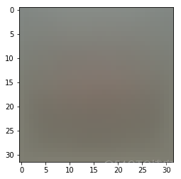
# Processing: subtract the mean images
mean_image = np.mean(X_train, axis=0)
plt.figure(figsize=(4,4))
plt.imshow(mean_image.reshape((32,32,3)).astype('uint8'))
plt.show()

X_train -= mean_image
X_val -= mean_image
X_test -= mean_image

# append the bias dimension of ones (i.e. bias trick)
X_train = np.hstack([X_train, np.ones((X_train.shape[0], 1))])
X_val = np.hstack([X_val, np.ones((X_val.shape[0], 1))])
X_test = np.hstack([X_test, np.ones((X_test.shape[0], 1))])
print('Train data shape: ', X_train.shape)
print('Validation data shape: ', X_val.shape)
print('Test data shape: ', X_test.shape)

Train data shape:  (49000, 3073)
Validation data shape:  (1000, 3073)
Test data shape:  (1000, 3073)

class LinearSVM(object):
    """ A subclass that uses the Multiclass SVM loss function """
    def __init__(self):
        self.W = None

    def loss_naive(self, X, y, reg):
        """
        Structured SVM loss function, naive implementation (with loops).
        Inputs:
        - X: A numpy array of shape (num_train, D) contain the training data
          consisting of num_train samples each of dimension D
        - y: A numpy array of shape (num_train,) contain the training labels,
          where y[i] is the label of X[i]
        - reg: float, regularization strength
        Return:
        - loss: the loss value between predict value and ground truth
        - dW: gradient of W
        """

        # Initialize loss and dW
        loss = 0.0
        dW = np.zeros(self.W.shape)

        # Compute the loss and dW
        num_train = X.shape[0]
        num_classes = self.W.shape[1] 
        for i in range(num_train):
            scores = np.dot(X[i], self.W)
            for j in range(num_classes):
                if j == y[i]:
                    margin = 0
                else:
                    margin = scores[j] - scores[y[i]] + 1    # delta = 1
                    if margin > 0:
                        loss += margin
                        dW[:,j] += X[i].T
                        dW[:,y[i]] += -X[i].T
        # Divided by num_train
        loss /= num_train
        dW /= num_train

        # Add regularization
        loss += 0.5 * reg * np.sum(self.W * self.W)
        dW += reg * self.W

        return loss, dW
    def loss_vectorized(self, X, y, reg):
        """
        Structured SVM loss function, naive implementation (with loops).
        Inputs:
        - X: A numpy array of shape (num_train, D) contain the training data
          consisting of num_train samples each of dimension D
        - y: A numpy array of shape (num_train,) contain the training labels,
          where y[i] is the label of X[i]
        - reg: (float) regularization strength
        Outputs:
        - loss: the loss value between predict value and ground truth
        - dW: gradient of W
        """

         # Initialize loss and dW
        loss = 0.0
        dW = np.zeros(self.W.shape)

        # Compute the loss
        num_train = X.shape[0]
        scores = np.dot(X, self.W)
        correct_score = scores[range(num_train), list(y)].reshape(-1, 1)    # delta = -1
        margin = np.maximum(0, scores - correct_score + 1)
        margin[range(num_train), list(y)] = 0
        loss = np.sum(margin) / num_train + 0.5 * reg * np.sum(self.W * self.W)

        # Compute the dW
        num_classes = self.W.shape[1]
        mask = np.zeros((num_train, num_classes))
        mask[margin > 0] = 1
        mask[range(num_train), list(y)] = 0
        mask[range(num_train), list(y)] = -np.sum(mask, axis=1)
        dW = np.dot(X.T, mask)
        dW = dW / num_train + reg * self.W

        return loss, dW

    def train(self, X, y, learning_rate = 1e-3, reg = 1e-5, num_iters = 100, 
             batch_size = 200, print_flag = False):
        """
        Train linear SVM classifier using SGD
        Inputs:
        - X: A numpy array of shape (num_train, D) contain the training data
          consisting of num_train samples each of dimension D
        - y: A numpy array of shape (num_train,) contain the training labels,
          where y[i] is the label of X[i], y[i] = c, 0 <= c <= C
        - learning rate: (float) learning rate for optimization
        - reg: (float) regularization strength
        - num_iters: (integer) numbers of steps to take when optimization
        - batch_size: (integer) number of training examples to use at each step
        - print_flag: (boolean) If true, print the progress during optimization
        Outputs:
        - loss_history: A list containing the loss at each training iteration
        """

        loss_history = []
        num_train = X.shape[0]
        dim = X.shape[1]
        num_classes = np.max(y) + 1

        # Initialize W
        if self.W == None:
            self.W = 0.001 * np.random.randn(dim, num_classes)

        # iteration and optimization
        for t in range(num_iters):
            idx_batch = np.random.choice(num_train, batch_size, replace=True)
            X_batch = X[idx_batch]
            y_batch = y[idx_batch]
            loss, dW = self.loss_vectorized(X_batch, y_batch, reg)
            loss_history.append(loss)
            self.W += -learning_rate * dW

            if print_flag and t%100 == 0:
                print('iteration %d / %d: loss %f' % (t, num_iters, loss))

        return loss_history

    def predict(self, X):
        """
        Use the trained weights of linear SVM to predict data labels
        Inputs:
        - X: A numpy array of shape (num_train, D) contain the training data
        Outputs:
        - y_pred: A numpy array, predicted labels for the data in X
        """

        y_pred = np.zeros(X.shape[0])
        scores = np.dot(X, self.W)
        y_pred = np.argmax(scores, axis=1)

        return

def loss_naive1(X, y, W, reg):
    """
    Structured SVM loss function, naive implementation (with loops).
    Inputs:
    - X: A numpy array of shape (num_train, D) contain the training data
    consisting of num_train samples each of dimension D
    - y: A numpy array of shape (num_train,) contain the training labels,
    where y[i] is the label of X[i]
    - W: A numpy array of shape (D, C) contain the weights
    - reg: float, regularization strength
    Return:
    - loss: the loss value between predict value and ground truth
    - dW: gradient of W
    """

    # Initialize loss and dW
    loss = 0.0
    dW = np.zeros(W.shape)

    # Compute the loss and dW
    num_train = X.shape[0]
    num_classes = W.shape[1] 
    for i in range(num_train):
        scores = np.dot(X[i], W)
        for j in range(num_classes):
            if j == y[i]:
                margin = 0
            else:
                margin = scores[j] - scores[y[i]] + 1    # delta = 1
                if margin > 0:
                    loss += margin
                    dW[:,j] += X[i].T
                    dW[:,y[i]] += -X[i].T
    # Divided by num_train
    loss /= num_train
    dW /= num_train

    # Add regularization
    loss += 0.5 * reg * np.sum(W * W)
    dW += reg * W

    return loss, dW

def loss_vectorized1(X, y, W, reg):
    """
    Structured SVM loss function, naive implementation (with loops).
    Inputs:
    - X: A numpy array of shape (num_train, D) contain the training data
    consisting of num_train samples each of dimension D
    - y: A numpy array of shape (num_train,) contain the training labels,
    where y[i] is the label of X[i]
    - W: A numpy array of shape (D, C) contain the weights
    - reg: (float) regularization strength
    Outputs:
    - loss: the loss value between predict value and ground truth
    - dW: gradient of W
    """

    # Initialize loss and dW
    loss = 0.0
    dW = np.zeros(W.shape)

    # Compute the loss
    num_train = X.shape[0]
    scores = np.dot(X, W)
    correct_score = scores[range(num_train), list(y)].reshape(-1, 1)    # delta = -1
    margin = np.maximum(0, scores - correct_score + 1)
    margin[range(num_train), list(y)] = 0
    loss = np.sum(margin) / num_train + 0.5 * reg * np.sum(W * W)

    # Compute the dW
    num_classes = W.shape[1]
    mask = np.zeros((num_train, num_classes))
    mask[margin > 0] = 1
    mask[range(num_train), list(y)] = 0
    mask[range(num_train), list(y)] = -np.sum(mask, axis=1)
    dW = np.dot(X.T, mask)
    dW = dW / num_train + reg * W

    return

from gradient_check import grad_check_sparse
import time

# generate a random SVM weight matrix of small numbers
W = np.random.randn(3073, 10) * 0.0001

# Without regularization
loss, dW = loss_naive1(X_val, y_val, W, 0)
f = lambda W: loss_naive1(X_val, y_val, W, 0.0)[0]
grad_numerical = grad_check_sparse(f, W, dW)

# With regularization
loss, dW = loss_naive1(X_val, y_val, W, 5e1)
f = lambda W: loss_naive1(X_val, y_val, W, 5e1)[0]
grad_numerical = grad_check_sparse(f, W, dW)

numerical: -8.059958 analytic: -8.059958, relative error: 6.130237e-11
numerical: -7.522645 analytic: -7.522645, relative error: 3.601909e-11
numerical: 14.561062 analytic: 14.561062, relative error: 1.571510e-11
numerical: -0.636243 analytic: -0.636243, relative error: 7.796694e-10
numerical: -11.414171 analytic: -11.414171, relative error: 1.604323e-11
numerical: 12.628817 analytic: 12.628817, relative error: 1.141476e-11
numerical: -9.642228 analytic: -9.642228, relative error: 2.188900e-11
numerical: 9.577850 analytic: 9.577850, relative error: 6.228243e-11
numerical: -5.397272 analytic: -5.397272, relative error: 4.498183e-11
numerical: 12.226704 analytic: 12.226704, relative error: 5.457544e-11
numerical: 14.054682 analytic: 14.054682, relative error: 2.879899e-12
numerical: 0.444995 analytic: 0.444995, relative error: 4.021959e-10
numerical: 0.838312 analytic: 0.838312, relative error: 6.444258e-10
numerical: -1.160105 analytic: -1.160105, relative error: 5.096445e-10
numerical: -3.007970 analytic: -3.007970, relative error: 2.017297e-10
numerical: -2.135929 analytic: -2.135929, relative error: 2.708692e-10
numerical: -16.032463 analytic: -16.032463, relative error: 1.920198e-11
numerical: 5.949340 analytic: 5.949340, relative error: 2.138613e-11
numerical: -2.278258 analytic: -2.278258, relative error: 6.415350e-11
numerical: 8.316738 analytic: 8.316738, relative error: 1.901469e-11

svm = LinearSVM()
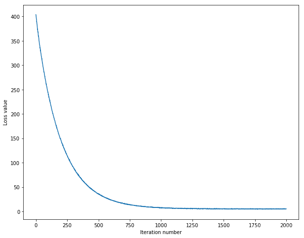
loss_history = svm.train(X_train, y_train, learning_rate = 1e-7, reg = 2.5e4, num_iters = 2000, 
             batch_size = 200, print_flag = True)

iteration 0 / 2000: loss 403.810828
iteration 100 / 2000: loss 239.004354
iteration 200 / 2000: loss 145.934813
iteration 300 / 2000: loss 90.564682
iteration 400 / 2000: loss 56.126912
iteration 500 / 2000: loss 36.482452
iteration 600 / 2000: loss 23.327738
iteration 700 / 2000: loss 15.934542
iteration 800 / 2000: loss 11.508418
iteration 900 / 2000: loss 8.614351
iteration 1000 / 2000: loss 7.845596
iteration 1100 / 2000: loss 6.068847
iteration 1200 / 2000: loss 6.017030
iteration 1300 / 2000: loss 5.407498
iteration 1400 / 2000: loss 5.282425
iteration 1500 / 2000: loss 5.760450
iteration 1600 / 2000: loss 4.764250
iteration 1700 / 2000: loss 5.395108
iteration 1800 / 2000: loss 5.025213
iteration 1900 / 2000: loss 4.858321

# Plot the loss_history
plt.plot(loss_history)
plt.xlabel('Iteration number')
plt.ylabel('Loss value')
plt.show()

# Use svm to predict
# Training set
y_pred = svm.predict(X_train)
num_correct = np.sum(y_pred == y_train)
accuracy = np.mean(y_pred == y_train)
print('Training correct %d/%d: The accuracy is %f' % (num_correct, X_train.shape[0], accuracy))

# Test set
y_pred = svm.predict(X_test)
num_correct = np.sum(y_pred == y_test)
accuracy = np.mean(y_pred == y_test)
print('Test correct %d/%d: The accuracy is %f' % (num_correct, X_test.shape[0], accuracy))

Training correct 18789/49000: The accuracy is 0.383449
Test correct 375/1000: The accuracy is 0.375000

learning_rates = [1.4e-7, 1.5e-7, 1.6e-7]
regularization_strengths = [8000.0, 9000.0, 10000.0, 11000.0, 18000.0, 19000.0, 20000.0, 21000.0]

results = {}
best_lr = None
best_reg = None
best_val = -1   # The highest validation accuracy that we have seen so far.
best_svm = None # The LinearSVM object that achieved the highest validation rate.

for lr in learning_rates:
    for reg in regularization_strengths:
        svm = LinearSVM()
        loss_history = svm.train(X_train, y_train, learning_rate = lr, reg = reg, num_iters = 2000)
        y_train_pred = svm.predict(X_train)
        accuracy_train = np.mean(y_train_pred == y_train)
        y_val_pred = svm.predict(X_val)
        accuracy_val = np.mean(y_val_pred == y_val)
        if accuracy_val > best_val:
            best_lr = lr
            best_reg = reg
            best_val = accuracy_val
            best_svm = svm
        results[(lr, reg)] = accuracy_train, accuracy_val
        print('lr: %e reg: %e train accuracy: %f val accuracy: %f' %
              (lr, reg, results[(lr, reg)][0], results[(lr, reg)][1]))
print('Best validation accuracy during cross-validation:\nlr = %e, reg = %e, best_val = %f'

lr: 1.400000e-07 reg: 8.000000e+03 train accuracy: 0.388633 val accuracy: 0.412000
lr: 1.400000e-07 reg: 9.000000e+03 train accuracy: 0.394918 val accuracy: 0.396000
lr: 1.400000e-07 reg: 1.000000e+04 train accuracy: 0.392388 val accuracy: 0.396000
lr: 1.400000e-07 reg: 1.100000e+04 train accuracy: 0.388265 val accuracy: 0.379000
lr: 1.400000e-07 reg: 1.800000e+04 train accuracy: 0.387408 val accuracy: 0.386000
lr: 1.400000e-07 reg: 1.900000e+04 train accuracy: 0.381673 val accuracy: 0.372000
lr: 1.400000e-07 reg: 2.000000e+04 train accuracy: 0.377531 val accuracy: 0.394000
lr: 1.400000e-07 reg: 2.100000e+04 train accuracy: 0.372735 val accuracy: 0.370000
lr: 1.500000e-07 reg: 8.000000e+03 train accuracy: 0.393837 val accuracy: 0.400000
lr: 1.500000e-07 reg: 9.000000e+03 train accuracy: 0.393735 val accuracy: 0.382000
lr: 1.500000e-07 reg: 1.000000e+04 train accuracy: 0.395735 val accuracy: 0.381000
lr: 1.500000e-07 reg: 1.100000e+04 train accuracy: 0.396469 val accuracy: 0.398000
lr: 1.500000e-07 reg: 1.800000e+04 train accuracy: 0.382694 val accuracy: 0.392000
lr: 1.500000e-07 reg: 1.900000e+04 train accuracy: 0.382429 val accuracy: 0.395000
lr: 1.500000e-07 reg: 2.000000e+04 train accuracy: 0.374265 val accuracy: 0.390000
lr: 1.500000e-07 reg: 2.100000e+04 train accuracy: 0.378327 val accuracy: 0.377000
lr: 1.600000e-07 reg: 8.000000e+03 train accuracy: 0.392551 val accuracy: 0.382000
lr: 1.600000e-07 reg: 9.000000e+03 train accuracy: 0.391184 val accuracy: 0.378000
lr: 1.600000e-07 reg: 1.000000e+04 train accuracy: 0.387939 val accuracy: 0.410000
lr: 1.600000e-07 reg: 1.100000e+04 train accuracy: 0.388224 val accuracy: 0.389000
lr: 1.600000e-07 reg: 1.800000e+04 train accuracy: 0.378102 val accuracy: 0.383000
lr: 1.600000e-07 reg: 1.900000e+04 train accuracy: 0.380918 val accuracy: 0.383000
lr: 1.600000e-07 reg: 2.000000e+04 train accuracy: 0.378224 val accuracy: 0.383000
lr: 1.600000e-07 reg: 2.100000e+04 train accuracy: 0.376204 val accuracy: 0.380000
Best validation accuracy during cross-validation:
lr = 1.400000e-07, reg = 8.000000e+03, best_val = 0.412000

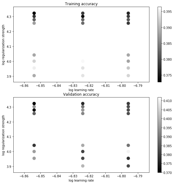
# Visualize the cross-validation results
import math

x_scatter = [math.log10(x[0]) for x in results]
y_scatter = [math.log10(x[1]) for x in results]

# Plot training accuracy
plt.figure(figsize=(10,10))
make_size = 100
colors = [results[x][0] for x in results]
plt.subplot(2, 1, 1)
plt.scatter(x_scatter, y_scatter, make_size, c = colors)
plt.colorbar()
plt.xlabel('log learning rate')
plt.ylabel('log regularization strength')
plt.title('Training accuracy')

# Plot validation accuracy
colors = [results[x][1] for x in results]
plt.subplot(2, 1, 2)
plt.scatter(x_scatter, y_scatter, make_size, c = colors)
plt.colorbar()
plt.xlabel('log learning rate')
plt.ylabel('log regularization strength')
plt.title('Validation accuracy')
plt.show()

# Use the best svm to test
y_test_pred = best_svm.predict(X_test)
num_correct = np.sum(y_test_pred == y_test)
accuracy = np.mean(y_test_pred == y_test)
print('Test correct %d/%d: The accuracy is %f' % (num_correct, X_test.shape[0], accuracy))

Test correct 369/1000: The accuracy is 0.369000

W = best_svm.W[:-1, :]    # delete the bias
W = W.reshape(32, 32, 3, 10)
W_min, W_max = np.min(W), np.max(W)
classes = ['plane', 'car', 'bird', 'cat', 'deer', 'dog', 'frog', 'horse', 'ship', 'truck']
for i in range(10):
    plt.subplot(2, 5, i+1)
    imgW = 255.0 * ((W[:, :, :, i].squeeze() - W_min) / (W_max - W_min))
    plt.imshow(imgW.astype('uint8'))
    plt.axis('off')
    plt.title(classes[i])
plt.show()

参考文献：

​​linear classification notes​​

更多AI资源请关注公众号：红色石头的机器学习之路（ID：redstonewill）